Graph

What is graph

• Wikipedia: A graph is a structure made of vertices and edges.
• I: Ok

A graph can be described as a way of representing relationships between things. For example, let’s consider the relationship of friends. A is a friend of B, B is a friend of C, and C is a friend of D. Additionally, D is a friend of A, and B. In this scenario, we refer to these individuals as vertices, and the connections between them as edges.

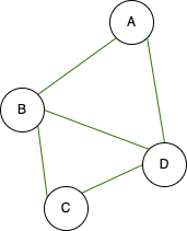
It can be described in this way. This graph is a connected graph with 4 vertices and 5 edges. A connected graph is a graph where every vertex is reachable from any other vertex through edges. We can observe the largest graph network on Facebook among friends.

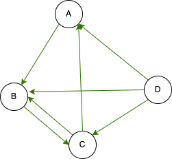
There is a slight difference in the relationship graph between Instagram and Twitter. Just because A follows B doesn’t necessarily mean that B follows A. For instance, in the scenario where A follows B, B follows C, C follows A and B, and D follows all of them.

Graph in computer

How can we save this structure to the computer? We have encountered various types of structures such as numbers, characters, arrays, and more. Now, let’s discuss how to save a graph using these structures.

Matrix

If the graph has N vertices, it can be represented by an NxN matrix or a 2-dimensional array. Each element A[i][j] in the matrix represents the presence or absence of a direct edge between the i-th vertex and the j-th vertex. If there is no edge, A[i][j] is 0, and if there is an edge, it can be assigned a value based on the weight of that edge in the case of a weighted graph.

The advantage is that we can immediately determine whether there is an edge between two vertices, and performing mathematical calculations becomes easier.

The drawback is that it can consume excessive memory. For instance, let’s consider a hypothetical scenario where a person can have a maximum of 5000 friends on Facebook. Considering the vast number of users in the billions, the matrix size will be much bigger than the total connections, and the majority of the matrix entries will be 0. In reality, we are not friends with everyone. Personally, I might be familiar with the names of around 300 individuals out of the 4 million people in Mongolia.

Adjacency vector

How can we reduce your memory usage? The matrix A is stored abstractly, where the array A[i] contains the list of vertices connected by a direct edge to the ith vertex. By adopting this approach, our memory consumption is reduced from N^2 to a number of edges. We can utilize a vector to store this information, as it allows for dynamic resizing, which is advantageous for our purposes.

Of course, using adjacency lists reduces memory consumption, but in some cases, it is not a very useful data structure. For example, we cannot determine immediately whether two vertices are connected.

Running over the graph

Of course, we can’t just describe it and leave it at that. There are many things you can do with a graph. For example, given a graph:

• How many different components does the graph have?
• given 2 vertices, what is the shortest path between them?
• Find all the possible vertices that can be visited starting from a single vertex.

There are many more topics to cover, so let’s dive into a few example scenarios.

BFS

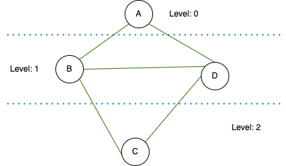
About BFS (Breadth First Search), the general idea is that the starting vertex is considered at level 0. Then, in the next step, all its neighboring vertices are considered at level 1. Similarly, the vertices connected to those neighbors are assigned level 2, and so on, as we traverse the graph. Each level represents the distance from the starting vertex.

Problem

Given a graph and two vertices, what is the shortest path between them?

We are starting from vertex X and our goal is to find the shortest path to vertex Y. At the beginning, X is considered to have traversed 0 paths, making it level 0. Now, what are the vertices called that have a level of 1? These vertices are directly connected to vertex X by an edge. As we move along these edges, we encounter paths numbered 1, which correspond to level 1. Moving further, level 2 consists of vertices that are directly connected to level 1 vertices. It’s important to note that if a vertex has already been encountered in a previous level, it should not be considered as level 2. Therefore, we assign a level value only to new vertices or vertices that haven’t been visited before.

By continuing this process from vertex X (level 0), we increment the levels until we reach vertex Y. The level assigned to vertex Y will represent the minimum path length from vertex X to vertex Y.

For simplicity, let’s consider the edges of the graph as pipes. Imagine that we have spilled water from vertex X. Initially, the water flows through all the pipes connected to vertex X. Then, it continues to flow through the pipes leading to the neighboring vertices. When the water reaches a vertex for the first time, it signifies that it has followed the shortest possible path from vertex X to that vertex. However, if the water has already reached that vertex before, it means that this path is redundant. The key concept here is to progress one level at a time, ensuring efficient traversal of the graph.

example BFS

How to write the code? We use the queue data structure (why not a vector or other structure?). A Queue is used, which consists of pairs. The first element of the pair represents the current vertex, and the second element represents the current level. Initially, we add the pair (X, 0) to the Queue.

To process the elements in the Queue, we perform the following steps:

1. Retrieve the first element from the queue, which is a pair (X, level).
2. Mark vertex X as visited, indicating that we have reached vertex X at level “level”. We don’t need to revisit this vertex again (no need to drain water). We save the water.
3. Add all the vertices directly connected to vertex X by an edge to the queue. Each vertex is added as a pair with the first element being the vertex itself, and the second element being level+1. This represents that these vertices are at the next level. After adding them, we increment the level.
4. Repeat steps 1-3 until we reach vertex Y. This algorithm finds the shortest path from a given vertex to all connected vertices.

By using this algorithm, we can efficiently find the shortest path from a starting vertex to all other vertices in the graph.

#include <queue>
#include <iostream>
using namespace std;
	
	int n, m;			
	bool vis[50000];		
	vector<int> adj[50000];		
	queue< pair<int,int> > q;

int main() {
	cin >> n >> m;	

	for(int i = 1; i <= m; i++) {
		int u, v;	
		cin >> u >> v;
		adj[u].push_back( v );
		adj[v].push_back( u );
	}
	int x, y;	
	
	cin >> x >> y;	

	q.push( make_pair( x, 0 ) );

	while( !q.empty() ) {	
		int nowU = q.front().first;	
		int nowW = q.front().second;
		
		vis[nowU] = 1;	

		if( nowU == y ) {
			cout << nowW << endl;	
			return 0;	
		}

		q.pop();	

		for(int i = 0; i < adj[nowU].size(); i++) {
			int v = adj[nowU][i];				
			if( !vis[v] ) {					
				q.push( make_pair( v, nowW+1 ) ); 	
			}
		}
	}
	cout << "Not connected!\n"; 	
	return 0;
}

DFS

I will write about DFS (Depth First Search), also known as the Depth-First Traversal algorithm. The main idea behind DFS is to start from a given vertex and explore as far as possible along each branch before backtracking. It starts by visiting the first neighboring vertex it encounters, then moves to the first neighboring vertex in that branch, and continues this process until it reaches a dead end or all vertices have been visited.

We can visualize this idea as a square maze, similar to those depicted in movies like The Shining, Pan’s Labyrinth, or Harry Potter and the Goblet of Fire. If we encounter a dead end, we backtrack and try another path. Unlike in real life, where it can be challenging to remember our exact steps, when working on a computer, we can keep track of our movements accurately.

In this code, DFS is implemented using recursion. Please try implementing it using a stack instead.

Problem

Given a graph, determine the number of components in the graph.

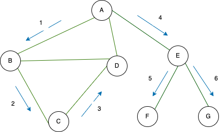
Let’s start by going from vertex 1 to the first adjacent vertex connected to it. Next, we’ll go to the first adjacent vertex connected to the previous vertex, excluding vertex 1. If we reach vertex 1 again, we’ll continue this process indefinitely. Now, what if, during this traversal, we have already visited all the vertices connected to a certain vertex before reaching that vertex? In that case, we’ll backtrack to the vertex we came from and move to the next unvisited adjacent vertex. We’ll repeat this process until we get stuck and backtrack again. By the time we finish, we will have visited all the vertices that are somehow connected to vertex 1. These vertices together form one connected component, which is referred to as the first component. If any vertex, denoted as the i-th vertex, does not belong to this component, then it is a separate component. We can find the connected component by performing a Depth-First Search (DFS) starting from this vertex.

DFS

#include <vector>
#include <iostream>
using namespace std;
	
	int n, m;		
	int comp;		
	bool vis[200000];		
	vector<int> adj[200000];	

void dfs(int u) {
	vis[u] = 1; 

	for(int v:adj[u]) {
		if( !vis[v] ) {
			dfs(v);
		}
	}
}

int main() {
	cin >> n >> m; 
	while( m-- ) {
		int u, v;	
		cin >> u >> v;
		adj[u].push_back( v );
		adj[v].push_back( u );
	}

	for(int i = 1; i <= n; i++) {
		if( !vis[i] ) {
			comp++;
			dfs( i );	
		}
	}
	cout << comp << endl; 
	return 0;
}

Summary

The graph is a vast field of study, and there is still much to explore regarding the relationship between edges and vertices. You can explore deeper into the concepts of dense and sparse graphs to gain a better understanding of their characteristics.

Please feel free to leave a comment if you spot any mistakes in the code or if you have any questions or thoughts to share.